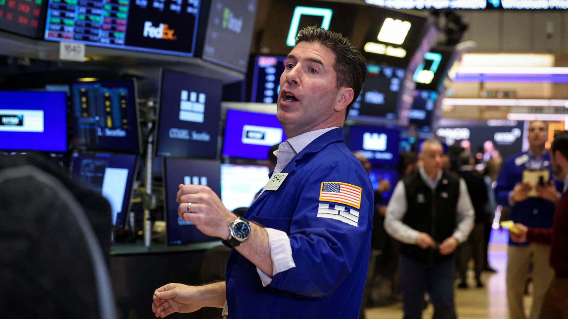
Traders work on the floor at the New York Stock Exchange (NYSE) in New York City, U.S., Feb. 27, 2026.
Brendan McDermid | Reuters
Stock futures tumbled in overnight trading after the U.S. and Israel attacked Iran over the weekend, causing oil prices to surge and adding an unstable Middle East to a list of growing worries for equity investors.
Futures on the Dow Jones Industrial Average dropped 571 points, or 1.2%. S&P 500 futures lost 1% and Nasdaq 100 futures declined a little more than 1%. Gold futures jumped 2% as investors piled into the global safe haven.
The joint U.S.-Israeli strikes killed Supreme Leader Ayatollah Ali Khamenei, marking a watershed moment for the Islamic Republic and one of its most consequential episodes since 1979. President Donald Trump told CNBC’s Joe Kernen that U.S. military operations in Iran are “ahead of schedule,” but investors are worried about a prolonged conflict despite those comments.
The large-scale assault was launched overnight Saturday after Iran refused American demands to curb its nuclear program. Iranian officials have vowed a forceful retaliation, raising fears the conflict could spread across the region.
“The tail risk of a sustained conflict is higher than in 2024 or 2025, though we don’t see this war escalating to a point where it drastically changes the US outlook,” said Barclays’ Ajay Rajadhyaksha in a note. But early this week “is too early to buy any dip, especially with investors used to a pattern of quick de-escalation.”
U.S. crude prices jumped 8% in early trading, as investors worry the confrontation could spiral into a broader war that disrupts supplies. Iran is the fourth-largest oil producer in OPEC, and uncertainty remains over who will ultimately govern the country amid the leadership vacuum.
The oil market’s trajectory may hinge on whether fighting disrupts traffic through the Strait of Hormuz, the world’s most important chokepoint for crude flows. A sustained interruption there could reverberate through global energy markets and reignite inflation pressures.
“Broader uncertainty suppresses investor sentiment, which can broadly weigh on risk-assets globally,” said Adam Hetts, global head of multi-asset at Janus Henderson. “In a prolonged period of uncertainty, increases in oil prices could generate a global inflationary scare.”
The geopolitical escalation compounds an already fragile backdrop for stocks. The S&P 500 sold off Friday and finished in the red for February amid renewed turmoil in artificial intelligence and software shares, as investors questioned whether rapid AI adoption could displace traditional software providers.
Fears that automation may erode business models and trigger mounting layoffs have weighed on sentiment, raising concerns about spillover effects on the broader economy.
“All told, we presume a shorter-term impact, but can’t rule out a more protracted friction to equities,” said Citi equity strategists in a note to clients about the Iran impact. “We also need to bucket this new volatility event alongside a growing list of concerns. Namely, the AI spending boom seems poised to persist, but the productivity promise is quickly facing off against AI-triggered business-model disruption.”