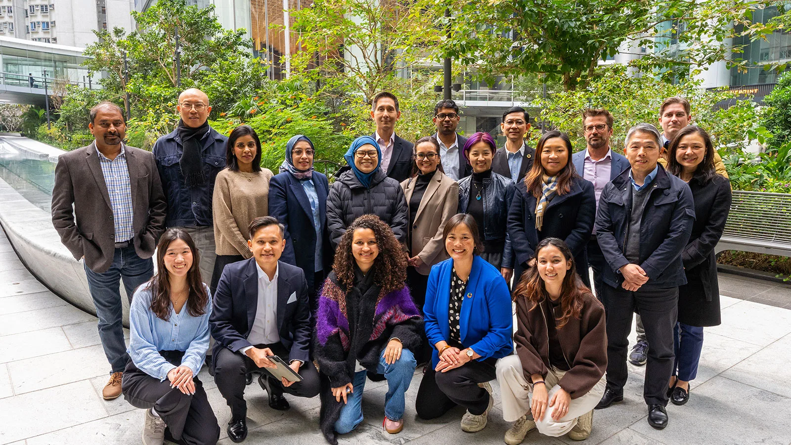
Category: 3. Business

• Gold eases after a four-day rally with prices stalling below $3,400 as bulls faced key resistance.
• US Treasury yields rise modestly, with the 10-year yield climbing from a three-month low ahead of the debt auction.
• US President Donald Trump revives tariff threats, targets pharma, semiconductors, India and Russia.

Gold (XAU/USD) edges higher on Wednesday after rebounding from an intraday low of $3,358, supported by a weaker US Dollar and subdued Treasury yields. At the time of writing, Gold is trading around $3,374 during American trading hours, though it continues to move within its broader weekly range, with bulls still struggling to clear the key $3,400 psychological barrier.

The yellow metal was on track to snap a four-day winning streak but recovered as the Greenback fell to a fresh weekly low, slipping below the lower end of its post-Nonfarm Payrolls (NFP) range. The rebound came as expectations for a Fed rate cut gained more momentum, giving the yellow metal fresh support.

Traders remain on the sidelines, refraining from placing aggressive bets as the market reassesses the Federal Reserve’s (Fed) monetary policy outlook. The latest batch of US economic data has cast doubts over the resilience of the world’s largest economy, reinforcing uncertainty ahead of the September policy decision. Still, the downside in Gold appears limited amid persistent global tariff tensions and firm market expectations that the Fed will lower interest rates next month.

Cautious sentiment also lingers as attention turns to the political shake-up at the Federal Reserve. The resignation of Fed Governor Adriana Kugler, effective August 8, has created a key vacancy on the Board. US President Donald Trump is expected to name her replacement by the end of the week.

Speculation over the potential nominees is fueling concerns that the Fed may tilt toward a looser monetary policy stance, particularly as President Trump has repeatedly stated that, in his view, interest rates should be cut. The move comes at a sensitive time, with markets already pricing in a high probability of a rate cut in September. Any sign of political influence over the Fed could inject fresh volatility into financial markets and reinforce safe-haven demand for Gold.

Market movers: US yields steady, ISM disappoints, Trump ramps up trade threats

• Minneapolis Fed President Neel Kashkari said the US economy is slowing, with signs of a cooling labor market, according to remarks made on CNBC. He reiterated that two rate cuts this year still seem appropriate, adding that it may be time to begin adjusting the policy rate in the near term. Kashkari also acknowledged uncertainty around the inflationary impact of new tariffs, noting it’s “still not clear” how they will feed through to price pressures. His comments add to the dovish tone from recent Fed speakers and further reinforce market expectations for a September rate cut.
• US Treasury yields edges slightly higher on Wednesday, paring recent losses after hitting multi-week lows. The 10-year yield, which dropped to a three-month low on Tuesday, currently trades around 4.236%, up 1.8 basis points on the day. The 30-year yield is also recovering, rising from a one-month low. It opened at 4.729% and is currently hovering near 4.813%, marking a gain of 8.4 basis points so far.
• The uptick in yields reflects a modest shift in sentiment as markets consolidate ahead of $42 billion 10-year note auction on Wednesday, which is expected to offer fresh clues on investor appetite for long-term US debt amid growing fiscal and geopolitical uncertainty.
• The ISM Services PMI for July fell to 50.1, missing expectations of 51.5 and slipping from 50.8 in June, signaling stagnation in the services sector.  While the headline reading still indicates marginal expansion, the details were more concerning. The Employment Index dropped deeper into contraction territory at 46.4, down from 47.2, highlighting ongoing labor market weakness. New Orders also declined to 50.3 from 51.3, pointing to fading demand.
• The Prices Paid Index in the ISM Services report rose to 69.9 in July from 67.1, marking its highest level since October 2022. The sharp rise in input costs, despite weakening activity, has reignited inflation concerns and highlighted persistent cost pressures across the services sector. These mixed signals have further clouded the Fed’s monetary policy outlook. According to the CME FedWatch Tool, markets are now assigning an 87% probability of a 25 basis point rate cut in September, with a total of 60 basis points of easing priced in by year-end.
• On the trade front, in an interview with CNBC, President Donald Trump said the tariffs on pharmaceutical imports will start with a modest rate and will go up in one year to 150% and up to 250%. He also confirmed that a separate announcement on semiconductors and chips will be made “in the next week or so.” During the interview, Trump also escalated his threats to impose higher tariffs against India for purchasing Russian Oil, saying he would “very substantially” raise tariffs on India within “the next 24 hours.”
• The Trump administration is also preparing new US sanctions targeting Russia’s secretive Oil tanker network comprising vessels with concealed ownership if President Vladimir Putin fails to agree to a ceasefire in Ukraine by Friday, as reported by the Financial Times.
• Earlier on Tuesday, President Trump confirmed that he was considering four candidates for Fed Chair, including Kevin Hassett and Kevin Warsh, and that Treasury Secretary Scott Bessent was not in the running as he “wants to stay in the Treasury.”
• Looking ahead, with no meaningful US data scheduled for release today, attention turns to remarks from several Fed officials. Fed Governor Lisa Cook and Boston Fed President Susan Collins are set to participate in a panel discussion, while San Francisco Fed President Mary Daly will speak at an economic summit.

Technical analysis: XAU/USD holds above 50-day SMA as momentum stalls near key resistance

Gold (XAU/USD) slips modestly on Wednesday, struggling to sustain momentum after stalling below the key $3,400 psychological barrier. The metal briefly broke below the ascending triangle’s lower trendline last week and found support just above the 100-day Simple Moving Average (SMA) at $3,282.

While the spot prices have since rebounded, the recovery was capped as prices were rejected at the broken triangle support, which is now acting as resistance.

The metal continues to consolidate just above the 50-day SMA near $3,346, which acts as immediate support, followed by the 100-day SMA. If prices break lower, the next targets could be around $3,200 and $3,150.

Momentum indicators remain mixed, reflecting indecision. The Relative Strength Index (RSI) on the daily chart sits at 52, hovering in neutral territory, suggesting neither bulls nor bears are in clear control.

Meanwhile, the Moving Average Convergence Divergence (MACD) indicator is showing early signs of recovery, with a minor bullish crossover and flattening histogram, indicating that bearish pressure may be fading.

A decisive daily close above the $3,390-$3,400 resistance band would invalidate the triangle breakdown and open the door for a potential run toward $3,450, with all-time highs around $3,500 back on the radar.

WhatsApp has taken down 6.8 million accounts linked to criminal scam centers worldwide, according to its parent company, Meta

NEW YORK — WhatsApp has taken down 6.8 million accounts that were “linked to criminal scam centers” targeting people online around that world, its parent company Meta said this week.

The account deletions, which Meta said took place over the first six months of the year, arrive as part of wider company efforts to crack down on scams. In a Tuesday announcement, Meta said it was also rolling new tools on WhatsApp to help people spot scams — including a new safety overview that the platform will show when someone who is not in a user’s contacts adds them to a group, as well as ongoing test alerts to pause before responding.

Scams are becoming all too common and increasingly sophisticated in today’s digital world — with too-good-to-be-true offers and unsolicited messages attempting to steal consumers’ information or money filling our phones, social media and other corners of the internet each day. Meta noted that “some of the most prolific” sources of scams are criminal scam centers, which often span from forced labor operated by organized crime — and warned that such efforts often target people on many platforms at once, in attempts to evade detection.

That means that a scam campaign may start with messages over text or a dating app, for example, and then move to social media and payment platforms, the California-based company said.

Meta, which also owns Facebook and Instagram, pointed to recent scam efforts that it said attempted to use its own apps — as well as TikTok, Telegram and AI-generated messages made using ChatGPT — to offer payments for fake likes, enlist people into a pyramid scheme and/or lure others into cryptocurrency investments. Meta linked these scams to a criminal scam center in Cambodia — and said it disrupted the campaign in partnership with ChatGPT maker OpenAI.

Data collection

Statistical data

This study collected agricultural statistical data at the national, provincial, prefectural, and county levels in China, covering the period from 1988 to 2022. The data sources include the statistical yearbooks from the National Bureau of Statistics of China (https://www.stats.gov.cn) and the Big Data Research Platform for China’s Economy and Society (https://data.cnki.net). Moreover, historical crop price records were obtained from the FAO (Food and Agriculture Organization of the United Nations) (https://www.fao.org/faostat)⁴¹. To evaluate irrigation and agricultural input levels, crop fertilizer application ratios were derived from the inventories of “Compilation of the National Agricultural Costs and Returns”⁴². Recommended fertilizer application ratios for different crops were obtained from He et al.⁴³. The proportion of irrigated land was obtained from the third simulation round of the Inter-Sectoral Impact Model Intercomparison Project (ISIMIP3a) dataset⁴⁴, which provides data on rainfed and irrigated cropland for crops from 1901 to 2021.

Spatial data

Several spatial datasets relevant to crop distribution, including land use, crop natural growth suitability, urban boundaries, and population density, have been used to facilitate the mapping of crop area. The land use data were employed to delineate the extent of cropland and irrigated cropland, including the China Land Cover Dataset (CLCD)⁴⁵, the China Land Use and Land Cover Remote Sensing Monitoring Dataset (CNLUCC)⁴⁶, the Global Land Cover Fine-Grained Classification Product (GLC_FCSD)⁴⁷, the China Arable Land Dataset (CACD)³, and the China Irrigated Cropland Dataset⁴⁸. The crop natural growth suitability and potential yield distribution were derived from the GAEZ v4 dataset⁴⁹. The population density data originated from the China Population Spatial Distribution Dataset⁵⁰. The urban extent data were obtained from the China Urban Boundary Dataset (GAIA)⁵¹. Additionally, the transport accessibility data were obtained from Weiss et al.⁵². All spatial datasets were rasterized and resampled to a 1-km resolution grid. The details of these datasets are provided in Table 1.

Modeling framework

The research framework is illustrated in Fig. 2, which consists of four key steps: pre-processing statistical and spatial data, allocating statistical harvest area data, validating the accuracy of the results, and analyzing spatiotemporal changes of crop patterns. First, national, provincial, and prefectural statistical data were harmonized and downscaled to grids, while county-level data were used to validate the accuracy of the mapping results. Then, crop cultivation was categorized into three different production systems, i.e., irrigated, high-input rainfed, and low-input rainfed based on crop irrigation and fertilizer application ratios. Multiple land use datasets were then integrated to develop a synthetic map of cropland and irrigated cropland. Meanwhile, pre-processing was performed on spatial datasets such as city boundaries, population distribution, and transportation accessibility (Figs. S1–S3). Then, a spatial allocation framework was used to downscale the prefecture-level crop area statistics into 1-km grids. Moreover, the accuracy of the dataset was evaluated in terms of both validation metrics and spatial patterns. Finally, changes in the spatiotemporal heterogeneity of crop distribution were analyzed.

Harmonization of statistical data

This study collected harvest area statistics for 16 different crop types across four different political administration levels. The detailed list of crop names is provided in Table 2. The time coverage of this built dataset spans from 1990 to 2020. We endeavored to collect crop statistics from publicly accessible sources, generally ensuring data completeness for major production regions (Fig. S4). However, due to the extended temporal coverage and reliance solely on public data, many regions inevitably have incomplete time series. To ensure data availability and methodological consistency, we followed previous studies by representing each time point with a 5-year average, using data from the two years before and after each time point^26,29,53,54. For instance, statistical values from 1988 to 1992 were utilized to map the crop patterns in 1990, while those from 2018 to 2022 were employed to map the crop patterns in 2020. Besides, the linear interpolation was used to fill the missing values. Due to the lack of prefecture-level statistical data for Xinjiang, Qinghai, and Xizang, spatial allocations for these provinces were based on provincial-level statistical data.

In order to ensure the consistency of statistical data across different administrative levels, this study used national-level statistical data as a benchmark and successively corrected for each province and prefecture. First, the crop harvest area for each province (({{HA}}_{j,t,p}^{{stat}})) was adjusted according to Eq. (1), based on the national total harvest area (({{HA}}_{j,t,{national}}^{{stat}})), resulting in the revised provincial harvest area denoted as ({{HA}}_{j,t,p}^{{revise}}):

where the j denotes the crop type, t represents the time node, and p indicates the provincial-level administrations. The sum of the revised area at the provincial level is highly in agreement with the national statistics, as shown in Fig. S5.

Based on the revised provincial-level data, a similar approach is applied to adjust the harvest area for the prefecture-level city (({{HA}}_{j,c}^{{stat}})) as Eq. (2):

where the (c) represents the prefecture-level city with province (p). The sum of the harmonized data at the prefecture level is equal to the revised provincial values, as shown in Fig. S6. Therefore, the total harmonized harvest area of all provinces and prefectures equals the national statistics.

Classification of crop production systems

Based on the ratios of irrigation and fertilizer application, each crop cultivation was categorized into three production systems: irrigated, high-input rainfed, and low-input rainfed. The proportion of irrigated crop for each 5-year node was extracted from the ISIMIP3a dataset⁴⁴. The proportions of high-input and low-input systems are determined based on actual crop fertilizer application statistics compared with the recommended amounts. The shares of irrigated system for crops (({H{A}_{{Ratio}}}_{j,t,p}^{{irrigat}{ion}})) are determined by averaging the gridded values at the prefecture level. Owing to the lack of crop fertilizer application data at the prefecture level, this study assumed that all prefectures within the same province share the same average fertilizer application ratios. The details of the crop production system classification are as follows.

First, the crop fertilizer application ratios of each province (({{Fert}}_{j,t,p}^{{unit}})) were obtained from the “Compilation of the National Agricultural Costs and Returns” as presented in Table S2. Then, the sum of fertilizer application for each crop (({{Fert}}_{j,t,p}^{{Sum}})) was calculated using Eq. (3). The average crop fertilizer applications for all provinces are shown in Table S3.

Then, the high-input production area of the crop (({{HA}}_{j,t,p}^{{high}})) is obtained from dividing the total fertilizer application by the recommended fertilizer application ratios for the crop (({{Fert}}_{j,p}^{{recommend}})), as shown in Eq. (4):

The ratios of high-input system in the total area (({H{A}_{{Ratio}}}_{j,t,p}^{{high}})) are calculated following Eq. (5):

Finally, the ratios of the low-input system (({H{A}_{{Ratio}}}_{j,t,p}^{{low}})) are calculated by subtracting the proportion of the irrigated and high-input area following Eq. (6). Tables S4–S6 show the detailed proportions for each production system.

Synthesis of cropland

The cropland distribution from different sources was synthesized using the multi-source data integration approach proposed by Lu et al.⁵⁵. The cropland extents were obtained from CACD, CLCD, GLC_FCSD, and CNLUCC datasets. The spatial resolutions of these datasets were resampled to 1 km, with temporal periods aligned to the time nodes of the statistics.

First, the average and maximum cropland areas for each grid were derived by spatially overlaying multiple datasets. Then, a ranking scoring table was developed to assess the credibility of the cropland distribution. As shown in Table S7, the agreement level reflects the degree of consensus among the datasets in classifying a grid cell as cropland. The rank value indicates the order of reliability across different data combinations. For example, an agreement level of 4 indicates that all datasets classify the grid cell as cropland; conversely, a value of 1 indicates that only one dataset identifies the cell as cropland. The ranking of the datasets was determined through existing data quality comparison studies and expert judgment. Given that the CACD was specifically developed for cropland mapping, it is considered to have the highest level of credibility⁵⁶. Additionally, comparative studies on data accuracy indicate that the CLCD demonstrates higher overall accuracy when compared to both the GLC_FCSD and the CNLUCC datasets^57,58. Finally, the synthesized average cropland area maps are illustrated in Fig. S7.

The approach for irrigated cropland synthesis is similar to cropland. The irrigated cropland maps were obtained from the China Irrigated Cropland Dataset, GLC_FCSD, and CNLUCC datasets. A scoring table for these irrigated cropland datasets is provided in Table S8. The synthesized maps of average irrigated cropland area for the period from 1990 to 2020 are shown in Fig. S8.

Spatial allocation of crop statistics

Prefecture-level statistics were allocated to 1-km grids using the maximum-score optimization approach developed by van Dijk et al.⁴⁰. This method builds upon the minimum cross-entropy framework originally proposed by You and Wood (2005, 2006)^31,32. The cross-entropy framework calculates the prior probability of crop distribution based on biophysical and socioeconomic factors, and then determines the actual probability under statistical constraints by minimizing cross-information entropy³³. To enable multi-temporal, high-resolution mapping, the maximum plant suitability score was used in place of the minimum cross-entropy metric, resulting in improved spatial resolution and faster convergence. The main steps of the model are described below.

First, the crop harvest area of the prefecture (({{HA}}_{j,t,c}^{{revise}})) is converted into the physical area (({{PA}}_{j,t,c})) based on crop planting intensity (({{CropIntensity}}_{j,t,c})) as expressed in Eq. (7). The assumption is that there is no difference in cropping intensity between prefectures within the same province. The average crop planting intensities for different crops are shown in Table S9.

Then, the crop plant suitability scores for different crop production systems (l) within the grid (i) are calculated. The irrigated and rainfed high-input systems are mainly located in large farms, and their score is influenced by both biophysical characteristics and socio-economic factors, including transport accessibility and crop prices. Therefore, their crop plant suitability score is presented as Eq. (8):

where the ({{access}}_{i}) represents the accessibility from the grid to cities, and where ({{rev}}_{{ijl}}) represents the economic benefit of the crop, which is calculated via Eq. (9):

where the ({{pot_yield}}_{i,j,l}) is the potential yield of crop (j) in grid (i) under (l) system, which is obtained from the GAEZ v4 dataset. The changes in crop prices (({{price}}_{j})) are shown in Table S10.

For rained low-input system, its plant suitability score is constrained mainly by the natural environment, which is calculated following Eq. (10):

The ({s{uit}{_index}}_{{ijl}}) denotes the plant suitability of crop (j) in grid (i) under (l) system, which is derived from the GAEZ v4 dataset as well.

Finally, based on the plant suitability scores of crops, the objective function designed to maximize the plant suitability score is formulated as Eq. (11):

The ({s}_{i,j,l}) represents the ratio of the area allocated to crop (j) under system (l) to the total area of the grid, which is the target solution value of the model. Meanwhile, the subsequent constraints should be abided by during the model-solving process as indicated in Eqs. (12–16).

1. 1.

   The area allocated to crops within the grid must not exceed the total area of the grid.

   $$0le {s}_{i,j,l}le 1,forall ,iforall ,jforall ,l$$

   (12)

2. 2.

   The cumulative ratios of different production systems within the grid must sum to 1.

   $$sum _{l}{s}_{i,j,l}=1,forall ,iforall ,j$$

   (13)

3. 3.

   The crop area is equal to the statistical data.

   $$sum _{l}{{PA}}_{j,c}times {s}_{i,j,l}={{PA}}_{j,c},forall ,i$$

   (14)

4. 4.

   The crop area does not exceed the total cropland area within the prefecture (({{cropland}{rm{_}}{area}}_{c})).

   $$sum _{l}{{PA}}_{j,l,c}times {s}_{i,j,l}le {{cropland}{rm{_}}{area}}_{c},forall ,iin c$$

   (15)

5. 5.

   The irrigated crop area does not exceed the total irrigated cropland area within the prefecture (({{irrigation_area}}_{c})).

To address data inconsistencies between different types of constraints, the slack variables are incorporated into the objective function. Higher weights (10⁶) are assigned to constraints relating to cropland availability and irrigated area to limit their slack, while lower weights (10⁵) are assigned to constraints relating to subnational statistics. This configuration ensures solution feasibility and quantitatively clarifies trade-offs in constraint prioritization^40,59. Furthermore, all weights, parameters, and implementation details have been made publicly available to enable rigorous validation and to ensure the robustness and reproducibility of the results.

The optimization model was implemented in the GAMS (General Algebraic Modeling System) using a linear programming framework, with the CPLEX (C-Simplex algorithm) solver employed to efficiently address large-scale spatial allocation problems. Data exchange between model components was managed by GDX (GAMS Data eXchange) format files. All data preprocessing and visualization procedures were performed in R⁶⁰. To improve allocation accuracy for China-specific crop patterns, we enhanced the original mapspamc package³⁸, thereby maintaining methodological consistency with global applications.

Validation metrics

The county-level statistics are used to evaluate the accuracy of the allocation results at the prefecture level. The scatter plot illustrates the relationship between the statistically derived harvest area (({{HA}}^{{stat}})) and the allocated harvest area (({{HA}}^{{alloc}})). Meanwhile, the Pearson correlation coefficient ((C{or})), the coefficient of determination (left({R}^{2}right)), and the root mean square error (({RMSE})) is used to quantitatively evaluate the accuracy of the results. The calculation methods for the different accuracy verification metrics are presented in Eqs. (17–19):

Analysis of crop distribution change

The Standard Deviation Ellipse (SDE) model was used to analyse the spatiotemporal evolution of crop area at 1-km resolution. The SDE effectively captures the directional trends of crop distribution and includes key elements such as the ellipse center, rotation angle, and semi-axes⁶¹. First, the center coordinates of the ellipse (left(bar{x},bar{y}right)) are calculated, weighted by the crop area in grid (i) across different years, as expressed in Eq. (20):

where the coordinates (({x}_{i},{y}_{i})) represent the location of grid (i) and the ({omega }_{i}) denotes the crop harvest area within that grid. Then, the rotation angle depicts the trend of crop distribution and is calculated following Eq. (21):

where (widetilde{x}) and (widetilde{y}) are the differences between the grid and center, indicating the displacements of the grid relative to the overall distribution. Finally, the standard deviations along the x-axis and y-axis are defined as the long semi-axis (({sigma }_{x})) and short semi-axis (({sigma }_{y})) as shown in Eqs. (22, 23):

Spatiotemporal changes of crop harvest area in China

China’s crop structure from 1990 to 2020 is shown in Fig. 3. It is clear that maize, rice, and wheat are the three dominant crops, together accounting for more than 65% of the total harvest area of crops. Their area shares decreased from 70.6% in 1990 to 67.3% in 2005 and then gradually increased to 72.1%. Meanwhile, the area of maize surpassed wheat and rice in 2005 and 2010 to become the largest crop in China. In contrast, the shares of rice and wheat decreased by 5.0% and 7.7%, respectively. Furthermore, the shares of non-staple crops such as soybeans, rapeseed, and groundnuts remained relatively stable during this period. In contrast, the harvest area of millet and sorghum decreased significantly. Among economic crops, the cotton area decreased from 4.7% in 1990 to 2.2% in 2020, while the tea area increased steadily from 0.7% to 2.1%. In addition, local cultivation crops, including tobacco, sugarbeet, sesame, sunflower, and sugarcane, have remained relatively marginal and stable over time.

Figure 4 shows the spatiotemporal changes in harvest area for four crops (maize, rice, wheat, and soybean) from 1990 to 2020. The center of crop harvest is gradually shifting northward, with the Northeastern China emerging as a critical region for agricultural production. The maize cultivation is concentrated in the Northern and Northeastern China (Fig. 4a). There has been a steady increase in the area under maize cultivation since 1900, with a particularly accelerated pace after 2005. In particular, the most significant maize expansion occurred in the Northeastern China, resulting in a shift of the center by approximately 214 kilometers to the northeast. Rice cultivation is concentrated mainly in the middle and lower reaches of the Yangtze River, followed by the Northeastern China (Fig. 4b). Between 1990 and 2000, a significant decline was observed in the Zhejiang and Jiangsu Provinces. In contrast, there was a notable expansion in the Northeastern China as well, resulting in a shift of about 344 kilometers to the northeast. The wheat cultivation is clustered in northern China, including Henan, Hebei and Shandong Provinces (Fig. 4c). As wheat production has become increasingly concentrated in the Huang-Huai-Hai Plain, the center of wheat production has shifted only 44 kilometers. Soybean cultivation is mainly concentrated in the Northeastern and Northern China (Fig. 4d). Heilongjiang and Inner Mongolia Provinces have been constantly extending their soybean area, resulting in a shift of the center by about 354 km to the northeast. The spatial distribution of non-staple crops exhibits significant heterogeneity, yet their primary cultivation centers are spatiotemporally stable (Fig. S9). For instance, rapeseed is predominantly concentrated in Central China (e.g., Hubei and Hunan provinces), whereas peanuts, millet, sunflower seeds, sorghum, and sesame are mainly cultivated in northern regions (e.g., Henan, Hebei, and Inner Mongolia). Furthermore, the primary harvest of potatoes, tea, sugarcane, and tobacco occurs in the southwestern provinces, including Yunnan, Guizhou, and Guangxi. Moreover, the primary production regions for cotton and sugar beet have shifted from North China to Xinjiang province.

6 August 2025

WindEurope statement on the second German offshore wind auction in 2025

Germany has announced the results of its second offshore wind auction in 2025. Two offshore wind sites in the North Sea with a total capacity of 2.5 GW were on offer. But the auction failed: not a single offshore wind project bid in. That’s a clear signal from the industry: Germany’s offshore wind auction design is not fit for purpose.

Germany’s second offshore wind auction round of 2025 was unsuccessful. Not a single offshore wind developer bid for either of the two sites N-10.1 and N-10.2. The sites in the German North Sea were centrally predeveloped and had a combined capacity of 2.5 GW.

Germany’s current offshore wind auction relies on negative bidding. It doesn’t offer any revenue stabilisation and exposes bidders to risks that go beyond their control. The uncapped negative bidding (“second bidding component”) further intensifies the financial pressure on offshore wind developers by asking them to pay high sums for the right to develop an offshore wind farm.

“The auction result must be a wake-up call for the German Government. Negative bidding adds costs that make offshore wind more expensive and reduces the number of companies willing and able to participate in auctions. It’s time to amend the auction model so Germany can deliver on its offshore wind targets and industrial competitiveness”, says Viktoriya Kerelska, Director of Advocacy & Messaging at WindEurope.

Most countries in Europe have introduced 2-sided Contracts for Difference (CfDs) as a revenue stabilisation mechanism for offshore wind development. CfDs mean lower financing costs and more visibility on future revenues. Denmark was the latest country to switch its auction framework to CfDs after its 3 GW negative bidding offshore wind tender didn’t attract any bids last December, similar to what happened now in Germany.

Germany is swimming against the tide. CfDs have proven to be the right model to finance offshore wind. They lower financing costs and deliver competitive electricity prices to society.

Wind energy already contributes 30% of all electricity consumed in Germany. It is the basis for competitive electricity prices for households and industry. It contributes to energy security in Germany as well as in wider Europe.

Dubai Aerospace Enterprise (DAE) Ltd on Wednesday announced a robust financial performance for the first half of 2025, driven by strategic acquisitions and operational efficiencies. The company reported a 24 per cent increase in revenue and a staggering 228 per cent rise in profit before tax compared to the same period last year.

According to the financial results for the six months ended June 30, 2025, DAE’s total revenue reached $843.6 million, up from $679.2 million in 2024. Profit before tax soared to $506.8 million, a significant jump from $154.3 million a year earlier. Operating cash flow also improved, rising to $659.0 million.

The company’s adjusted pre-tax profit margin increased to 25.7 per cent, while its adjusted pre-tax return on equity climbed to 13.3 per cent, reflecting enhanced profitability and capital efficiency.

Major acquisition boosts fleet and revenue

A key driver of DAE’s performance was the $2.0 billion acquisition of Nordic Aviation Capital (NAC), completed in May 2025. The deal expanded DAE’s fleet by nearly 50 per cent, bringing the total to approximately 750 aircraft. The acquisition included 236 aircraft (230 owned and 6 managed), and DAE sold 35 aircraft during the period.

CEO Firoz Tarapore commented, “The acquisition of NAC has significantly strengthened our market position. We’ve already integrated front-office operations and expect full integration of back-office systems by the end of this quarter.”

Tarapore also highlighted the impact of refinancing and cost-cutting measures, which contributed to the surge in profitability. “Our capital adequacy, funding, and liquidity metrics remain very strong,” he added.

Engineering division delivers strong growth

DAE Engineering, operating under the Joramco brand, also posted impressive results. Revenue rose 26 per cent to $119 million, while profitability jumped 80 per cent to $39.1 million. The division logged approximately 924,000 man-hours and completed 143 maintenance checks in the first half of the year.

Check before travelling to airport, Birmingham Airport sayspublished at 15:06 British Summer Time

15:06 BSTBreaking

Here’s the full statement from Birmingham Airport, published a short time ago on X:

“Following an aircraft incident, the runway is temporarily closed.

“We apologise for the inconvenience this will cause.

“We will keep passengers already at the airport informed and those due to travel later today are advised to check the status of their flight before coming to the airport.

“We will continue to issue updates when we can.”

Manure from cows and pigs is a surprisingly large source of greenhouse gases (GHGs) in the United States — over 1% of the country’s total emissions. The vast majority (about 80%) of these emissions are methane, with the rest coming from nitrous oxide.

Most dairy and swine farms in the U.S. currently manage manure using “wet systems.” These use water jets to flush manure into storage structures such as lagoons or tanks, creating a liquid or slurry. Wet storage systems create ideal conditions for methane-producing microorganisms to thrive, allowing them to emit large quantities of the gas into the atmosphere.

Methane is over 80 times more potent than carbon dioxide over a 20-year period, and reducing it is one of the fastest ways to slow global warming. Yet current efforts to tackle manure methane are lagging in the U.S., both in terms of testing and adoption. It is time to widen the lens and invest in a broader set of solutions for manure methane — solutions that can offer tangible benefits for farmers as well as the climate. Our new analysis provides a close look at both the problem and potentially promising solutions.

US Manure Emissions Are Underestimated — and Rising

The U.S. Environmental Protection Agency (EPA) estimates that manure management contributes around 1.3% of the country’s total GHG emissions, with most of this coming from dairy and swine operations. But recent satellite data shows that methane emissions are being undercounted in the U.S. livestock sector.

Our own analysis suggests that methane emissions from dairy and swine manure may be at least 40% higher than EPA estimates. This reflects more recent data from the 2022 U.S. Census of Agriculture, which shows that herd sizes are growing, and how that impacts manure storage systems. As livestock operations continue to consolidate and increase in herd size, they become more reliant on storing manure in liquid form, generating more methane. This means manure emissions will likely keep rising unless targeted action is taken.

Biogas Digesters Are Not a Universal Solution

Biogas digesters are currently a leading solution to reduce methane emissions from livestock manure. In the dairy sector, more than 11% of manure is now treated in digesters. These systems capture biogas (a mixture of methane and carbon dioxide) during manure storage and convert it into either electricity or vehicle fuel, popularly called “renewable natural gas.” But while they receive the most policy and financial support, digesters offer only modest methane reductions from manure itself. Most of their climate benefits come from offsetting fossil fuel emissions by generating energy, rather than directly reducing emissions from manure storage.

The main concern is what happens after digestion. Most digesters in the U.S. remove less than a third of the methane-generating material from manure. The leftover material, known as “digestate,” is typically stored in uncovered lagoons or pits that continue to emit methane into the atmosphere. Without gas-tight storage or additional treatment, much of the benefit of methane capture is lost. This means that digesters reduce methane from manure storage by only about 25%. The benefits may rise to 35% if the digestate is stored in covered, gas-tight systems that prevent further methane release.

Methane can also leak from other parts of the digester system, including the cover, biogas flaring units, feedstock tanks and gas upgrading equipment. Most digesters in the U.S. are not designed to fully break down manure or to manage emissions from digestate. They operate with relatively short treatment times and typically lack sealed storage. This results in lower methane reductions and additional environmental trade-offs, such as increased ammonia and nitrous oxide emissions when digestate is stored or applied as fertilizer in crop fields.

Cost is another challenge. Digesters are expensive to purchase and operate, often costing over $500 per cow, per year. This may be financially feasible for farms that have thousands of animals. But without policy support and subsidies, digesters are prohibitively expensive for small and medium farms and substantially increase the costs of milk or pork production.

These limitations underscore the need to strengthen measurement, monitoring, reporting and validation for existing digesters. Better data can help identify underperformance, detect methane leaks and ensure systems operate as intended.

However, given the high cost and relatively low overall mitigation potential of biogas digesters, manure management interventions should also begin shifting toward more efficient and cost-effective alternatives.

Alternative Technologies Show Promise, but Need More Support

Compared to anaerobic digesters, other technologies — including solid-liquid separation, aeration and acidification — offer more cost-effective options for manure methane mitigation. These approaches often cost less than $80 per cow, per year, and can be applied across various farm sizes, making them more versatile than large-scale digesters. Yet despite their practical advantages, they have received limited policy and funding support.

Solid-liquid Separation

Most methane from manure storage is emitted by the breakdown of methane-producing solids under wet, oxygen-free (“anaerobic”) conditions. Solid-liquid separation reduces emissions by removing a large share of these solids before the manure is stored. The solids, once separated, are drier and more exposed to air, inactivating methane-producing microorganisms. The remaining liquid has far fewer methane-producing solids and, therefore, releases much less methane during storage in lagoons or tanks.

Mechanical equipment such as screw presses, screens or centrifuges can be used to perform this separation on the farm. Depending on the separation system used, methane emissions from manure storage can be reduced by up to 65%. Solid-liquid separation also helps reduce odor, improves the fertilizer value of manure, and prevents solids from accumulating in storage lagoons (which reduces the maintenance cost of removing sludge).

Yet adoption remains limited. Cost is partly to blame: While solid separators are significantly cheaper than anaerobic digesters, they still require upfront investment in equipment, installation and maintenance, and few programs offer financial or technical support to help farmers adopt them. California’s Alternative Manure Management Program has supported the installation of several solid separators in the state. However, while USDA offers cost-share programs for general manure management, states rarely provide targeted support for non-digester technologies.

In addition, farmers don’t have a clear picture of the return on investment. More detailed quantification of solid separators’ economic value — including cost savings from bedding, improved lagoon function and nutrient recovery — could help make a stronger case for adoption.

Manure Acidification

Another promising technology is acidification, or mixing manure with an acid. Acidic manure creates unfavorable conditions for methane-forming microorganisms, thereby reducing methane emissions. This approach is most commonly used in Denmark as part of the country’s ammonia control regulation.

Literature strongly supports the use of acidification to reduce methane, nitrous oxide and ammonia emissions. However, the extent of these benefits depends on the frequency, type and dosage of the acid used. Researchers report up to an 89% reduction in methane using higher acid doses and a 46% reduction with lower doses of acid. While other methane-reduction methods (including anaerobic digestion and solid-liquid separation) can risk increasing nitrous oxide emissions, acidification stands out as the only approach consistently shown to reduce both nitrous oxide and ammonia emissions alongside methane.

Our analysis shows that acidification can be implemented at a much lower cost than most other manure mitigation technologies. We also found that it is easier to integrate into small and medium-sized farm operations with minimal changes to existing practices. However, there is virtually no farm-level data on its effectiveness in the U.S., and only a few trials are underway.

A technology this promising warrants more pilot projects and on-farm trials. These trials should assess effectiveness as well as practical barriers — such as odor, infrastructure corrosion risk and safety concerns — while quantifying co-benefits, like ammonia reduction. Engaging farmers early in the process will be key to building collective trust and informing adoption.

Manure Aeration

Manure aeration involves bubbling air through manure storage using a circulator or pump. The presence of oxygen creates “aerobic” conditions that suppress methane-producing microbes. Complete aeration, where manure is continuously mixed with air over extended periods, can virtually eliminate methane emissions. However, this approach is energy-intensive and costly, requiring continuous operation of pumps or blowers. As a more affordable alternative, partial aeration involves introducing air intermittently or targeting only a portion of the storage volume. While less intensive, partial aeration can still reduce methane emissions by 40% to 57% and may be more feasible for many farms.

Beyond methane mitigation, aeration offers several practical benefits for farmers. It helps reduce odor by minimizing the smelly byproducts of anaerobic decomposition. It also improves manure handling by breaking down solids into a more uniform slurry that requires less agitation before land application.

Aeration has been widely used for decades in wastewater treatment to manage human waste, but it’s rarely used on livestock farms, likely due to high operating costs. Still, it may be a good fit for swine farms, where manure is often stored in deep pits that are compatible with aeration systems. Aeration is less practical for very large farms that use lagoons, as it becomes more expensive and less efficient at that scale.

While manure aeration has not been widely adopted, advancements in system design and components are starting to make it a more attractive option by lowering costs, improving energy efficiency, and making systems easier to operate and maintain. Some farmers are recognizing the value proposition of aeration, particularly in terms of odor control and ease of manure pumping.

Comparing Manure Methane Mitigation Options

Manure management option	Methane mitigation potential	Cost per dairy cow, per year
Anaerobic digestion	25% to 35% (manure storage emissions only)	$317 to $643
Solid-liquid separation	12% to 65%	$3 to $24
Acidification	46% to 89%	$6 to $20
Aeration	40% to 57%	$24 to $79

^{Note: Cost estimates are preliminary.}

Adoption Is Limited by Funding and Field Data

Despite promising results in early trials, alternatives to biogas digesters remain underused on U.S. farms. A key barrier is the lack of farm-scale data to build confidence in how these technologies perform in real-world conditions. Most evidence comes from international case studies or controlled trials, leaving major information gaps regarding costs, emissions outcomes and day-to-day management needs in the U.S.

At the same time, limited funding and narrow eligibility requirements prevent many farmers from accessing the support they need to adopt these technologies. Most manure-related funding is concentrated on large-scale biogas systems. Alternatives that may work better for small- and mid-sized farms receive little attention, few incentives, and limited technical assistance and training. As a result, the most accessible and potentially cost-effective solutions remain out of reach for most producers.

Bringing Solutions to Farmers

Cost and technical barriers aside, on-farm solutions will not work without farmer buy-in. Methane reductions will contribute to a more stable climate and improved agricultural outcomes in the long term. However, farmers often do not see these technologies as offering immediate financial gains or increased productivity. This can make widespread adoption challenging, especially among those managing tight budgets and unpredictable incomes.

The good news is that these technologies can offer tangible benefits for farmers. For instance, solid-liquid separation can provide practical and financial advantages: Reducing lagoon volume lowers cleanout frequency and cost; enhancing fertilizer value allows more targeted nutrient use and reduces the need for synthetic fertilizers; and separated solids can be reused as animal bedding, avoiding additional purchases. Acidification can reduce ammonia levels in the air, which can lower respiratory stress for animals and promote better health for workers and nearby communities.

Promoting these co-benefits and boosting adoption will require involvement from a wide range of stakeholders, including farmers, extension specialists, manure services contractors, companies with food and agriculture supply chains, and policymakers.

• Farmer associations can help raise awareness and connect members to available incentive programs or pilot opportunities.
• Companies with food and agriculture supply chains aiming to reduce scope 3 emissions can support adoption by engaging their suppliers, incorporating these practices into their procurement standards, funding trials through supplier programs, and participating in broader partnerships.
• Policymakers and funders should prioritize grant programs and public-private partnerships that support on-farm trials, technical training and open sharing of results.
• Manure services contractors will play a central role in implementing technologies like acidification. They should be engaged early through training, equipment support, and targeted incentives to help deliver solutions that work in practice.
• Environmental organizations and governments will need to work together to coordinate these efforts, helping to simultaneously reduce GHG emissions from manure management and improve economic benefits for farmers. They can also help ensure that tools and standards are in place to measure and track emissions reductions across various systems in a consistent way.

Manure management is a growing climate challenge that demands more scalable and cost-effective solutions. While digesters have dominated investment in the U.S., their high costs and limited effectiveness underscore the need for alternatives. Promising options like solid-liquid separation, acidification and aeration offer potential for meaningful methane reductions and some on-farm benefits. Yet these technologies remain underutilized and still involve net costs. Expanded piloting is needed to evaluate real-world performance and economic viability. Broader adoption will require targeted financial incentives, and private sector investment will be essential to accelerate progress.

To learn more, read our new working paper.

The Islamabad IT Park, a state-of-the-art facility in Chak Shehzad, is scheduled for inauguration in Q3 2025. The facility covers 720,000 sq. ft., aims to create 7,500 jobs, and will boost IT exports by US$70 million. To foster innovation and entrepreneurship, the park will include startup incubation centers and a full business support center.

This support center will provide legal, marketing, and financial advisory services to growing businesses and startups. Moreover, the park will include research and development labs and virtual classrooms for technology-driven learning and innovation.

An industry-academia linkage center will enable collaboration between universities, researchers, and IT industry professionals. This will help bridge the gap between academic research and commercial technology ventures in the country.

A key highlight is Pakistan’s first-ever Tier III data center, offering uninterrupted power, robust data security, and high reliability with 99.982% uptime. This advanced data center will support secure hosting, high-performance computing, and reliable cloud services. Therefore, it is expected to attract global tech companies to Pakistan’s digital ecosystem.

The government has prioritized early completion of the project, with round-the-clock construction underway. Infrastructure development is central to the government’s strategy for expanding the ICT sector in Pakistan.

The Islamabad IT Park is a landmark project reflecting a strong commitment to national digital transformation. The park is poised to become a dynamic hub for IT professionals, startups, and global tech companies alike, helping to position Pakistan as a leading center for ICT services and helping expand Pakistan’s tech ecosystem.